6章 学習に関するテクニック

6.1 パラメータの更新

6.1.1 冒険家の話

6.1.2 SGD

mutable struct SGD
    lr::Float
end
SGD() = SGD(0.01)

function update(self::SGD, params, grads)
    for (key,_)=params
        params[key] .-= self.lr * grads[key]
    end
end

～

network = TwoLayerNet(...)
optimizer = SGD()

for i = 1:10000
    ...
    x_batch, t_batch = get_mini_batch(...) # ミニバッチ
    grads = gradient(network, x_batch, t_batch)
    params = network.params
    update(optimizer, params, grads)
    ...
end

～

6.1.3 SGDの欠点

6.1.4 Momentum

～

mutable struct Momentum # """Momentum SGD"""
    lr::AbstractFloat
    momentum::AbstractFloat
    v
end
 Momentum(lr=0.01, momentum=0.9) = Momentum(lr, momentum, nothing)
         
function update(self::Momentum, params, grads)
    if isnothing(self.v)
        self.v = IdDict()
        for (key, val) = params
            self.v[key] = zero(val)
        end
    end

    for (key,_) = params
        self.v[key] = self.momentum .* self.v[key] .- self.lr * grads[key] 
        params[key] .+= self.v[key]
    end
end

～

6.1.5 AdaGrad

～

mutable struct AdaGrad # """AdaGrad"""
    lr::AbstractFloat
    h
end
AdaGrad(lr=0.01) = AdaGrad(lr, nothing)
        
function update(self::AdaGrad, params, grads)
    if isnothing(self.h)
        self.h = IdDict()
        for (key, val) = params
            self.h[key] = zero(val)
        end
    end

    for (key,_) = params
        self.h[key] .+= grads[key].^2
        params[key] .-= self.lr * grads[key] ./ (sqrt.(self.h[key]) + 1e-7)
    end
end

～

6.1.6 Adam

6.1.7 どの更新手法を用いるか？

6.1.8 MNISTデータセットによる更新手法の確認

6.2 重みの初期値

6.2.1 重みの初期値を0にする？

6.2.2 隠れ層のアクティベーション分布

import OrderedCollections: OrderedDict
using Plots

function sigmoid(x)
    return 1 / (1 + exp(-x))
end

node_num = 100              # 各隠れ層のノード（ニューロン）の数
hidden_layer_size = 5       # 隠れ層が5層
activations = OrderedDict() # ここにアクティベーションの結果を格納する

for i = 1:hidden_layer_size
    if i != 1
        x = activations[i-1]
    else
        x = randn(1000, 100)
    end

    w = randn(node_num, node_num) * 1


    z = x * w
    a = sigmoid.(a) # シグモイド関数！
    activations[i] = a
end

～

# ヒストグラムを描画
p = []
for (i, a) = activations    
    push!(p, histogram!(a[:], bins=30, xlim=(0,1), title="$i-layer", leg=false))
end
plot(p..., layout=(1,length(activations)))

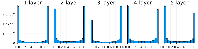
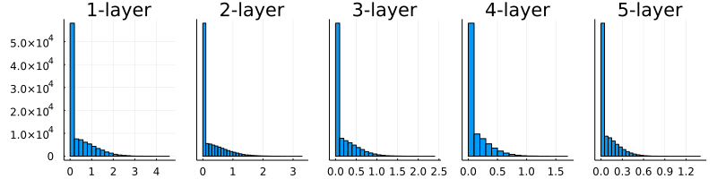
図6-10　重みの初期値として標準偏差1のガウス分布を用いたときの、各層のアクティベーションの分布

～

# w = randn(node_num, node_num) * 1
w = randn(node_num, node_num) * 0.01

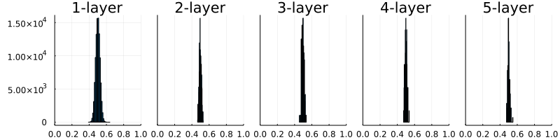
図6-11　重みの初期値として標準偏差0.01のガウス分布を用いたときの、各層のアクティベーションの分布

～

node_num = 100  # 前層のノードの数
w = randn(node_num, node_num) / sqrt(node_num)

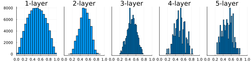
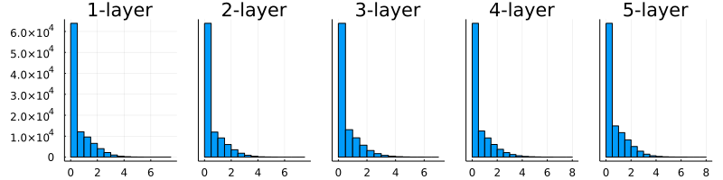
図6-13　重みの初期値として「Xavierの初期値」を用いたときの、各層のアクティベーションの分布

～

6.2.3 ReLUの場合の重みの初期値

～

6.2.4 MNISTデータセットによる重み初期値の比較

6.3 Batch Normalization

6.3.1 Batch Normalization のアルゴリズム

6.3.2 Batch Normalization の評価

6.4 正則化

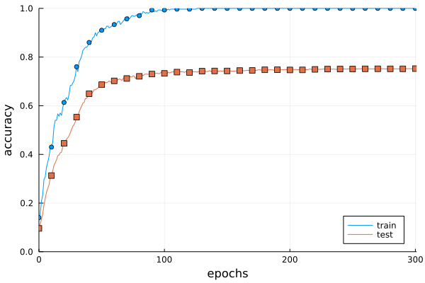
6.4.1 過学習

(x_train, t_train), (x_test, t_test) = load_mnist(normalize=true)

# 過学習を再現するために、学習データを削減
x_train = x_train[1:300, :]
t_train = t_train[1:300]

～

network = MultiLayerNet(784, [100, 100, 100, 100, 100, 100], 10,
                        weight_decay_lambda=weight_decay_lambda)
optimizer = SGD(0.01) # 学習係数0.01のSGDでパラメータ更新

max_epochs = 201
train_size = size(x_train, 1)
batch_size = 100

train_loss_list = zeros(0)
train_acc_list = zeros(0)
test_acc_list = zeros(0)

iter_per_epoch = max(train_size / batch_size, 1)
epoch_cnt = 0

for i = 0:1000000000
    batch_mask = shuffle(1:train_size)[1:batch_size]
    x_batch = x_train[batch_mask, :]
    t_batch = t_train[batch_mask]

    grads = gradient(network, x_batch, t_batch)
    update(optimizer, network.params, grads)

    if i % iter_per_epoch == 0
        train_acc = accuracy(network, x_train, t_train)
        test_acc = accuracy(network, x_test, t_test)
        append!(train_acc_list, train_acc)
        append!(test_acc_list, test_acc)

        global epoch_cnt += 1
        if epoch_cnt >= max_epochs
            break
        end
    end
end

～

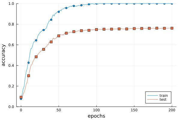
図6-20　訓練データ（train）とテストデータ（test）の認識精度の推移

～

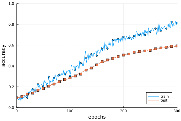
6.4.2 Weight decay

～

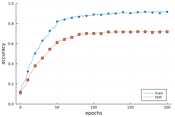
図6-21　Weight decayを用いた訓練データ（train）とテストデータ（test）の認識精度の推移

～

6.4.3 Dropout

～

mutable struct Dropout
    dropout_ratio::AbstractFloat
    mask
end

function Dropout(dropout_ratio=0.5)
    return Dropout(dropout_ratio, nothing)
end

function forward(self::Dropout, x, train_flg=true)
    if train_flg
        self.mask = rand(eltype(x), size(x)) .> self.dropout_ratio
        return x .* self.mask
    else
        return x * (1.0 - self.dropout_ratio)
    end
end

function backward(self::Dropout, dout)
    return dout .* self.mask
end

～

～

6.5 ハイパーパラメータの検証

6.5.1 検証データ

～

(x_train, t_train), (x_test, t_test) = load_mnist(normalize=true)

# 訓練データをシャッフル
x_train, t_train = shuffle_dataset(x_train, t_train)

# 検証データの分割
validation_rate = 0.20
validation_num = round(Int, size(x_train, 1) * validation_rate)

x_val = x_train[1:validation_num, :]
t_val = t_train[1:validation_num]
x_train = x_train[validation_num:end, :]
t_train = t_train[validation_num:end]

～

6.5.2 ハイパーパラメータの最適化

6.5.3 ハイパーパラメータの最適化の実装

～

weight_decay = exp10(rand()*((-4)-(-8))+(-8))
lr = exp10(rand()*((-2)-(-6))+(-6))

～

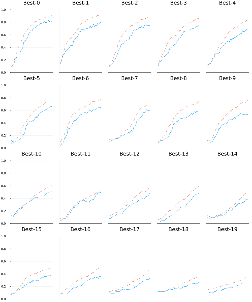図6-24　実線は検証データの認識精度、点線は訓練データの認識精度

～

Best-1 (val acc : 0.82) | lr:0.009260488167935177, weight decay:5.434206992791276e-5
Best-2 (val acc : 0.8) | lr:0.009792286718596086, weight decay:2.8153724279336563e-6
Best-3 (val acc : 0.75) | lr:0.007121165304873689, weight decay:2.203068790227544e-7
Best-4 (val acc : 0.74) | lr:0.007906392853673758, weight decay:7.987884306758652e-8
Best-5 (val acc : 0.69) | lr:0.005874541870339833, weight decay:5.256434391633917e-6

～

6.6 まとめ

～